New window utility in MS Office

Sometimes our task requires constantly moving between two ends of the same Excel sheet or between two separate sheets of the workbook. It is time consuming and downright irritating. However, MS Excel has already provided us with amazing feature called New Window to deal with this.

So how this utility helps us? Clicking on new window will open the same workbook in a different window. This will allow us to refer to the sheets in our workbook from a separate window and excuse us from navigating the same sheet. This new window is actually just another view of the current file. It’s not a different version of the current file. So, any changes made in the current window will be reflected in the new window as well and vice-versa. You don’t need to save changes made in the new window separately! And MS Excel doesn't ask you to save separately also.

Let's try to understand this using an example. We are working on an excel file in which data is given on two different sheets, as shown below

So we have file named 'eg' in which we have data sets on two different sheets. I need to use the data from sheet 2 in sheet 1 and to make the whole work simple, I will make use of New Window feature. 

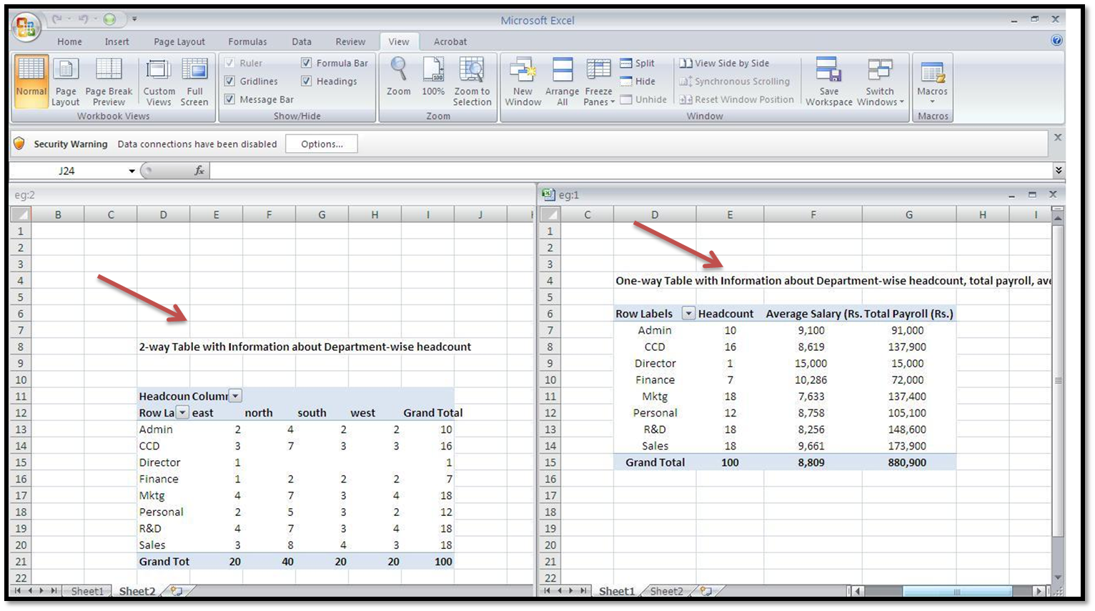
When I click on VIEW > NEW WINDOW, something like this happens

A new window opens up. The original file is renamed 'eg1' while the new file in the new window is named 'eg2'. So, the workbook name is followed by a number, making it easier to access them. 

So have you noticed? You can now bypass a series of CTRL + Page Up or Page Down keystrokes by using this tool! All you need to press is ALT + Tab or CTRL + Tab to shuffle between the two windows!

We can easily perform functions like data comparison or movement of data through the new window.

You can create multiple new windows of a file, however, we recommend current window and one new window to avoid confusion.

For best results, you can use this tool with the View Side by Side (or Arrange all (Horizontally or vertically) as shown below

Different Cell Editing Modes in MS Excel

Do you often face problem 

while editing a large formula in Excel?

                     or

dealing with values in different cells while preparing charts?

The above two problems might look little different, but their solution lies in knowing one very important feature of MS Excel that few have an idea about - Cell editing modes. 

Have you ever noticed a word written on the bottom left corner of the Excel workbook when you open it for the first time? Or when you start writing in a cell? If you haven't done so, try it now. You will be seeing the words 'Ready' and 'Enter' as shown in the screenshots below. 

They show the particular mode the cell is in. 

One beautiful aspect of MS Excel is that it allows users to have a lot of flexibility when it comes to editing and navigating. Now let’s explore how different cell modes help us in editing the data effectively.

Any excel cell can be in one of the three modes – Ready, Edit and Enter & Point. By default an excel cell is always in ready mode. It allows you to enter any data in any cell. This is the first cell mode. Pressing F2 once will change the mode to Edit and doing so twice will lead to the third mode i.e. Enter & Point. Now let us try to understand these modes with the help of an example.

We have a set of data as shown below

We are in the Ready mode and that has allowed us to input the data in various cells.  Now I wish to edit the formula cell (7.9 %). So I click on that cell and then press F2. 

Now we are in the Edit mode and can make any modifications inside the cell. Remember that pressing arrow key won’t take you to the next cell now. Instead, the cursor will keep moving in the same cell. 

Please note that when you are in Edit or Entry mode, most of the tabs and buttons will be disabled. You can use them only when you go back to Ready mode

Now I want to add the value of one more cell in the formula, but I can’t do it in Edit mode as my movement is restricted to the selected cell only. So I will press F2 once more to move to Enter & Point mode. 

Often, while entering a large formula, we need to navigate the whole sheet to add different values. The third mode, Enter & Point, comes handy in situations like these. Now we are ready to navigate the sheet to add the desired value in the formula. 

As I begin to navigate the sheet, the mode changes to Point from Enter. In this mode the particular data cell that you have ‘pointed to’ is shown in dotted lines. For instance in the above example I wish to insert the value of 8 % in the formula and so I have pointed to that cell. 

There are few important points worth noting here. Remember that many keyboard shortcuts don’t work in edit mode. You need to go back to Ready mode for that to happen. Also, you can return to the default mode of Ready from any mode by hitting Esc key. 

In the next article we will learn about new window utlity

How Quick Access Toolbar makes even shortcuts shorter

Now let’s see how Quick Access Toolbar can make some shortcuts redundant with the help of an example. 

In a workplace we often end up getting a file that has been poorly drafted. Before we move on with our work, it becomes necessary to do a bit of formatting and editing on the file. For example, consider the following –

It is clear from the screenshot that we need to adjust the column width to give the data a clean and proper look. Now this can be done in two ways –

a) Adjusting the width by dragging the boundary of the concerned column.

b) Using the following shortcut – ALT > H > O > I

Any of the above will do the job. But you will have to repeat it every time the column or row entries needed adjustment. This is where the quick access toolbar comes handy. All you need to do is add ‘Autofit Column Width’ from the list of commands on the toolbar. 

Now select the concerned column as shown below

Click on the shortcut for Autofit Column Width on the quick access toolbar and voila! Your job is done in a single click. Isn't it wonderful?

Similarly you can shorten several long shortcuts to make your working on Excel even easier and faster.

In our next article we will be learning about different cell editing modes. 

10 important ALT based shortcuts in MS Excel

Shortcut Keys	Description
Alt > A > S	Opens the sort dialogue box
Alt > A > T	Applies filters on data or removes filters
Alt > A > G > G	Groups the data (in rows or columns)
Alt > M > P or Alt > M > D	Traces precedent cells or dependent cells of an active cell
Alt > W > VG	Removes the grid lines from active sheet
Alt >W > F	Freezes/unfreezes view panes.
Alt > H > I > R	Inserts a new row above the current one
Alt > H > O >I	Auto fits the column width to suit the length of text in your column
Alt > H > V > S	Opens the Paste Special dialogue box
Alt > H > 9 or Alt > H > 0	Reduces decimal places or increases decimal places respectively

All versions of MS Office applications have prompted users to use more of the keyboard. If you just press ALT in MS Office application, you will notice that all tabs get highlighted with an alphabet. If you then press any alphabet highlighting a tab, you are directed to that tab and all buttons in that tab now get highlighted with different alphabet or group of alphabets.

For example, if we now press H, we will be seeing the following highlighted tabs on the excel sheet

Just keep on following this path to reach your desired button (or tool) using ALT.

Please note that these shortcuts are not a combination of keys like the CTRL based shortcuts. They are a sequence of keys. i.e. there is no need to juggle around by simultaneously pressing 2 or 3 keys. Instead, after pressing ALT, keys are hit in a sequence(steps) to accomplish a particular function.

E.g. Just press ALT, [leave it], then press M to go to Formulas tab, [leave it]

Doesn't this make life much easier when using ALT shortcuts? Further, you don’t need to remember the shortcuts, as MS Office keeps on prompting you for the next step!! Like this, you can navigate and use all utilities and tools in MS Excel, MS Word or other MS Office applications

Note that with Office 2007 onward, you can create your own shortcuts for tools and buttons that you use frequently! This is possible by customizing the Quick Access Toolbar or Tabs. We’ll cover this in our next article. 

Important formatting and editing shortcuts in MS Excel

Shortcut Keys	Description
Ctrl + Shift + ~/$/3/%/!	Allows you to change the formats as follows
Ctrl + Shift + ` (or ~ button)	Excel Default format (general number)
Ctrl + Shift + 1 (or ! button)	Comma (Thousand, million separator) and Decimal format
Ctrl + Shift + 3 (or # button)	Date format (dd-mm-yy)
CTRL + Shift + Home	(Currency format)
Ctrl + Shift + 5 (or % button)	(Percentage format)
Hiding and unhiding Rows and Columns
CTRL+ 9/CTRL + shift + 9		Hide/Unhide the row
CTRL+ 0/CTRL + shift + 9		Hide/Unhide the column
Drawing and removing outline borders, quickly
CTRL + Shift + &		Makes outline border for selected cells
CTRL + Shift + _		Removes all the lines, outline boarders in your selection
CTRL + D/R		Fills cells Down/Right

Have you noticed that you get ‘#VALUE!’ error when you work with dates in Excel? Or sometimes you are performing date based calculations and you get numbers! Or sometimes you have to quickly get a percentage format or change % format into the regular Excel default format.

Formatting is necessary to showcase or present the data in the intended manner. Without formatting the information generated through the data may be misconstrued. An example of formatting is changing the format of the value in a cell from a general number (78406) to the comma and decimal format (784,406.00). This is needed when we want to show a huge value precisely, like in the case of a company’s balance sheet.

Often we find formatting a headache due to the efforts we have to put in. Formatting shortcuts come handy for us here as hitting few keys only will do the necessary job.

An Example for understanding the shortcuts for changing the format

Let’s try to understand with the help of an example. Suppose we have imported some data from another file as shown below. The data consists of the current market capitalization of 5 firms. 

As we can see above, the values are given in two different formats. We wish to have these values in currency format. So, first of all we will select all the values and then use the shortcut Ctrl + Shift + 4 

As we can see above, the values are in their correct format now with commas & decimals. In this way we can change any data in the desired format using shortcuts. 

Hiding and unhiding Rows and Columns

Upon using CTRL + 9 the row, in which the selected cell is located, disappears. It is a straightforward action. However, unhiding the same row later requires little more knowledge than just knowing the shortcut. To unhide the row you first need to select the rows next to the hidden row. Then use the shortcut (CTRL + Shift + 9) to reveal the hidden row. The same theory applies to the hidden column. 

Shortcut for filling cells Down/Right 

Now Ctrl +D/R, a shortcut to fill cells Down/Right is also a very useful shortcut as it saves 50% of time in a copy-paste operation (Ctrl + C and Ctrl + V). This is how it works!

a. Select the area where you wish to paste the content (destination area) starting with source cell. Then press Ctrl + D or Ctrl + R

b. If you don’t select the destination area and just press Ctrl + D in the source cell, it will copy and paste the details in the cell immediately below.

c. Note that it fills the cells with content and formatting (cell comments are not copied)

Now that you have learnt the important formatting skills, it is time to teach your co-workers too how to format a file in short time easily. It will eventually ease your burden only, isn’t it?

Our next article will be the final article in the series of shortcuts for Excel and will help you make the use of shortcuts easier.  

5 important selection shortcuts in MS Excel

Shortcut Keys	Description
Shift/CTRL + Space	Allows you to select the entire row/column
Shift + Arrow Key	Extends the selection by one cell
CTRL + A	Selects entire range in a table or the entire worksheet
CTRL + Shift + Arrow keys	Extends the selection to the last non-blank (filled) cell in the same column or row as the active cell
CTRL + Shift + Home	Extend the selection from currently active cell to the beginning of the worksheet i.e. Cell A1

Whenever you will be working on MS excel, there will always be need of selecting data for copy-pasting or highlighting or other editing purpose. Sometimes you may have to select only few specific cells from a large number of cells. Selection shortcuts make this task very easy for you. In the table we have discussed in brief the 6 most important selection keys.

1. Shift/CTRL + Space - The combination of Shift with space key will select the entire row your selected cell is located in. Similarly pressing control key with space will select the entire column. 

2. Shift + Arrow Key - Use this shortcut to select the adjacent cell in any direction i.e. to the left/right/up/down. 

3. CTRL + A - If pressed inside a table (A range or array of adjoining filled cells), the entire range is selected. If pressed once more, the entire worksheet will be selected.

4. CTRL + Shift + Arrow keys - This shortcut performs the action of selection till last filled cell in a row/column

An example will help you understand how to use the above mentioned shortcut

As we can see above, the excel file in question lists the batting stats of all those batsmen who have scored 2,000 or more in the test matches. It consists of more than 250 players and we need to select the data pertaining to all of them. So using mouse and dragging it to select the data is really a bad idea. Instead, we will be using the shortcuts to accomplish the task in just 2 steps. 

In first step we will be using CTRL + Shift + right arrow to select the first row till the last filled cell as shown below

Now, in the second step, hit CTRL + Shift + down arrow. This will complete our job of selecting all the data from the workbook as shown below

Did you notice how we were able to select the whole data set in couple of seconds and that too without any fuss? 

Here are few important points worth noting

a. Remember that if you press spacebar in a cell it is considered as a filled (non-blank) cell, as Space is considered as a character. 

b. Ctrl + A can also be used to select the whole data given in a tabular form.  The point to be noted here is that using this shortcut will also select the column numbers and the particulars in this example as they are part of the data table. So this shortcut can’t be used for selective selection. 

Now that you have learnt to select the data swiftly and easily without using a mouse, why don’t you show the co-workers the magic of your fingers and earn their adulation. 

In our next article we will be dealing with important formatting shortcuts. 

5 important navigation shortcuts in MS Excel

Shortcuts make the work on MS Excel a lot easier. You may have noticed, as you shuffle lesser between mouse and keyboard, your speed of work grows manifold. Navigation within a sheet or between different worksheets, Excel files and other applications is a part of our daily working and so the navigation keys have a huge role to play in optimizing our efficiency. In the table we have highlighted 5 very important navigation shortcuts. 

Let's go through these shortcuts in brief and understand with the help of examples. 

1. ALT + Tab / Windows Logo + Tab - This shortcut allows switching between different open applications on your system. Kindly note that Windows logo can be used for switching only in Windows 7 and above. 

2. CTRL + Tab - With few clicks you can navigate between the multiple open excel files using this shortcut. 

3. CTRL + Page up/Page Down - Similarly you can easily move between different sheets of the same workbook through this shortcut. 

4. Ctrl + Arrow keys - This shortcut allows you to go to the next filled cell/last cell in the row or column. With just the arrow keys & CTRL, you can navigate across the entire worksheet that has over 16,000 columns and a million rows, as shown below. 

5. ALT + F4 - The day has ended and it is time to turn your machine off. There is no need to close all the open Excel files individually. This shortcut will close the application along with the files. 

So next time, don’t touch the mouse when you have to navigate, save a bit of time, reach home earlier and give a pleasant surprise to your family!

Our next article will be addressing the data selection issues in Excel and the shortcuts to tackle them. Keep visiting this page for the latest articles.